MDL Network Backbones

Tutorial

Code to perform network backboning method derived in “Fast nonparametric inference of network backbones for weighted graph sparsification” (Kirkley, 2024, https://arxiv.org/abs/2409.06417).

The function allows for both directed and undirected networks and provides options to adjust the analysis according to the network’s characteristics.

elist: A list consisting of directed tuples $(i, j, w_{ij})$ representing edges from node $i$ to node $j$ with weight $w_{ij}$ .
directed: Specify whether the input edge list is directed or undirected.
out_edges: Determine whether to track out-edges or in-edges attached to each node in the local pruning method.
allow_empty: Decide whether to allow empty backbones when the minimum description length is achieved with no edges.

Outputs include the global and local network backbones along with their inverse compression ratios:

backbone_global: Edge list of the global MDL-optimal backbone.
backbone_local: Edge list of the local MDL-optimal backbone.
compression_global: Inverse compression ratio for the global backbone.
compression_local: Inverse compression ratio for the local backbone.

The method minimizes the following MDL objectives according to Eq. 1 and Eq. 5 in https://arxiv.org/abs/2409.06417:

Microcanonical Global Description Length Objective of Network Backbone:

$\mathcal{L}_M^{(\text{global})}(G^{(b)}) = \log (E+1) + \log (W-E+1) + \log \binom{E}{E^{(b)}} +\log \binom{W^{(b)}-1}{E^{(b)}-1} +\log\binom{W-W^{(b)}-1}{E-E^{(b)}-1}$

Microcanonical Local Description Length Objective of Network Backbone:

$\mathcal{L}_M^{(\text{local})}\left(G^{(b)}\right) = \log\binom{N+W-E-1}{W-E} + \sum_{i=1}^{N} \Bigg(\log(k_i + 1) + \log(s_i - k_i + 1) + \log \binom{k_i}{k_i^{(b)}} + \log \binom{s_i^{(b)} - 1}{k_i^{(b)} - 1} + \log \binom{s_i - s_i^{(b)} - 1}{k_i - k_i^{(b)} - 1} \Bigg)$

MDL Backboning

This module provides functions to calculate the MDL-optimal network backbones for both global and local perspectives.

Functions
Function	Description
logchoose(n, k)	Compute the logarithm of the binomial coefficient.
logmultiset(n, k)	Compute the logarithm of the multiset coefficient.
to_undirected(edge_list, policy=”sum”)	Convert a directed edge list to an undirected edge list by merging edges.
MDL_backboning(elist, directed=True, out_edges=True, allow_empty=True)	Compute the MDL-optimal global and local network backbones.

Reference

function logchoose(n, k) [source]

Description: Compute the logarithm of the binomial coefficient.

Parameters:

(n, k)

n: Total number of items.
k: Number of chosen items.

Returns:

float: Logarithm of the binomial coefficient.

function logmultiset(n, k) [source]

Description: Compute the logarithm of the multiset coefficient.

Parameters:

(n, k)

n: Number of types.
k: Number of items.

Returns:

float: Logarithm of the multiset coefficient.

function to_undirected(edge_list, policy="sum") [source]

Description: Convert a directed edge list to an undirected edge list by merging edges.

Parameters:

(edge_list, policy="sum")

edge_list: List of directed edges as tuples (i, j, w_ij).
policy: Policy for merging edges, can be "sum", "max", "min", or "error". Defaults to "sum".

Returns:

list: Undirected edge list as tuples (i, j, w_ij) where edges are merged according to the specified policy.

function MDL_backboning(elist, directed=True, out_edges=True, allow_empty=True) [source]

Description: Compute the MDL-optimal global and local network backbones from the given edge list.

Parameters:

(elist, directed=True, out_edges=True, allow_empty=True)

elist: List of edges as tuples (i, j, w_ij).
directed: Boolean indicating if the network is directed, defaults as `True`.
out_edges: Boolean indicating whether to track out-edges (`True`) or in-edges (`False`), defaults as `True`.
allow_empty: Allows empty backbones if `True`, defaults as `True`.

Returns:

backbone_global: Edge list of the global MDL-optimal backbone.
backbone_local: Edge list of the local MDL-optimal backbone.
compression_global: Inverse compression ratio for the global backbone.
compression_local: Inverse compression ratio for the local backbone.

Demo

Example Code

Step 1: Import necessary libraries

import networkx as nx
import matplotlib.pyplot as plt
from paninipy.mdl_backboning import MDL_backboning

Step 2: Define the weighted edge list

# Weighted edge list for the example
elist = [
    (0, 1, 12), (0, 3, 20), (0, 4, 8),
    (1, 2, 1), (1, 4, 3),
    (2, 0, 1), (2, 1, 3),
    (3, 2, 3), (3, 4, 1),
    (4, 3, 1)
]

Step 3: Compute backbones and compression ratios

# Compute backbones using out-edges
backbone_global, backbone_local, compression_global, compression_local = MDL_backboning(
    elist, directed=True, out_edges=True
)

Step 4: Visualize the original network and backbones

def visualize_backbones(elist, backbone_global, backbone_local, compression_global, compression_local):
    G_original = nx.DiGraph()
    G_global = nx.DiGraph()
    G_local = nx.DiGraph()

    for i, j, w in elist:
        G_original.add_edge(i, j, weight=w)
    for i, j, w in backbone_global:
        G_global.add_edge(i, j, weight=w)
    for i, j, w in backbone_local:
        G_local.add_edge(i, j, weight=w)

    pos = nx.spring_layout(G_original, seed=42)
    W_original = sum([d['weight'] for u, v, d in G_original.edges(data=True)])
    E_original = G_original.number_of_edges()

    W_global = sum([d['weight'] for u, v, d in G_global.edges(data=True)])
    E_global = G_global.number_of_edges()

    W_local = sum([d['weight'] for u, v, d in G_local.edges(data=True)])
    E_local = G_local.number_of_edges()

    plt.figure(figsize=(18, 6))

    plt.subplot(1, 3, 1)
    nx.draw_networkx_nodes(G_original, pos, node_color='lightblue', node_size=500)
    nx.draw_networkx_edges(G_original, pos, arrowstyle='->', arrowsize=15)
    nx.draw_networkx_labels(G_original, pos)
    plt.title('Original Network')
    plt.axis('off')
    plt.text(0.5, -0.1, f'Total weight of the network = {W_original}\nTotal number of edges = {E_original}', ha='center', transform=plt.gca().transAxes)

    plt.subplot(1, 3, 2)
    nx.draw_networkx_nodes(G_global, pos, node_color='red', node_size=500)
    nx.draw_networkx_edges(G_global, pos, arrowstyle='->', arrowsize=15)
    nx.draw_networkx_labels(G_global, pos)
    plt.title('Global Backbone')
    plt.axis('off')
    plt.text(0.5, -0.1, f'Total weight of the network = {W_global}\nTotal number of edges = {E_global}\nInverse compression ratio = {compression_global:.4f}', ha='center', transform=plt.gca().transAxes)

    plt.subplot(1, 3, 3)
    nx.draw_networkx_nodes(G_local, pos, node_color='lightgreen', node_size=500)
    nx.draw_networkx_edges(G_local, pos, arrowstyle='->', arrowsize=15)
    nx.draw_networkx_labels(G_local, pos)
    plt.title('Local Backbone')
    plt.axis('off')
    plt.text(0.5, -0.1, f'Total weight of the network = {W_local}\nTotal number of edges = {E_local}\nInverse compression ratio = {compression_local:.4f}', ha='center', transform=plt.gca().transAxes)
    plt.tight_layout()
    plt.savefig("mdl_network_backbones.png", bbox_inches='tight', dpi=200)
    plt.show()

visualize_backbones(elist, backbone_global, backbone_local, compression_global, compression_local)

Example Output

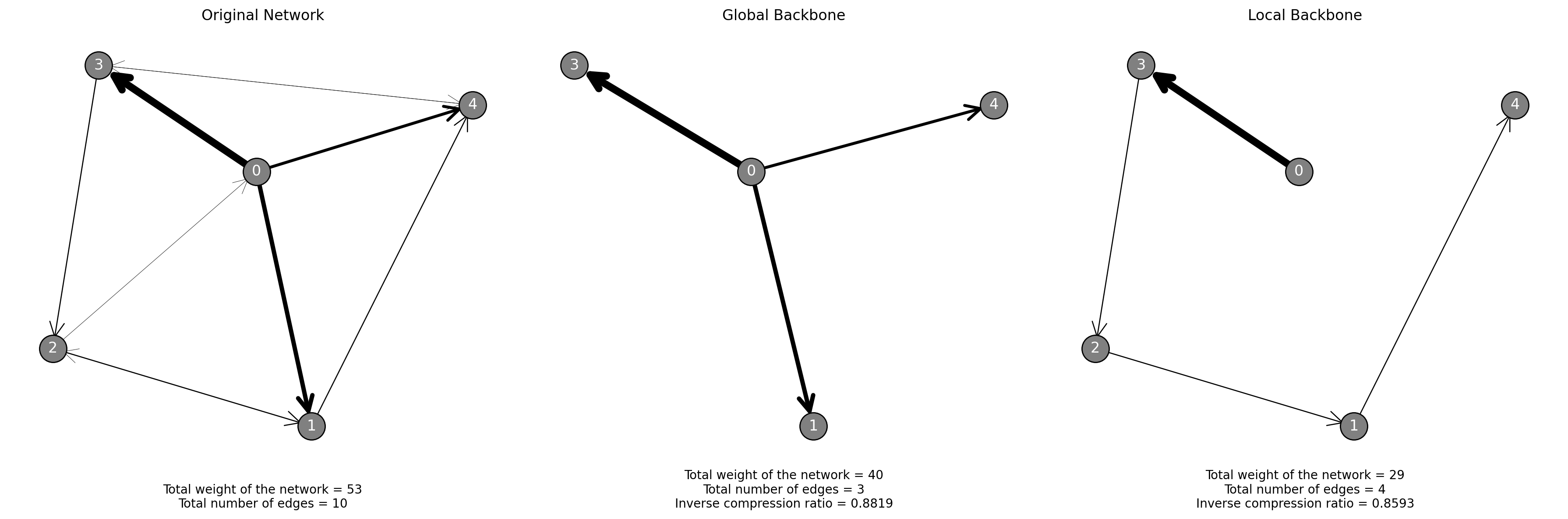
Visualization of the original network and the extracted backbones with statistics.

Left: Original weighted, directed network, with edge width proportional to weight. Center: Global MDL backbone, which learns a global threshold on the edge weights for network sparsification. Right: Local MDL backbone using out-neighborhoods. The local MDL method learns a threshold adapted to each neighborhood’s weight heterogeneity. Summary statistics are shown below each network.

Paper Source

If you use this algorithm in your work, please cite:

A. Kirkley, “Fast nonparametric inference of network backbones for weighted graph sparsification.” arXiv preprint arXiv:2409.06417 (2024). Paper: https://arxiv.org/abs/2409.06417